generalized-multilevel-networks
Source:vignettes/generalized-multilevel-networks.Rmd
generalized-multilevel-networks.RmdPresentation of generalized multivel networks
This vignette shows how to use the MLVSBM package to
deal with generalized multilevel networks. This is done by modeling
these networks with an ad-hoc Stochastic Block Model. The
mathematical details can be found at http://www.theses.fr/en/2022UPASM005
(Chapter 2.E).
A diagonal acyclic graph of the model for a graph with \(L\) levels is provided below.
        A^1             A^{L-1}
         |               |
         v               v
Z^1 --> Z^2 --> ... --> Z^L
 |       |               |
 v       v               v
X^1 --> X^2 --> ... --> X^L
A temporal network with the same nodes at each time is a particular case of generalized multilevel networks with diagonal affiliation matrices.
Description of the data
Assume that we have a generalized multilevel networks with \(4\) levels, each between \(80\) and \(100\) nodes and \(3\) latent blocks. The description of the levels are the following:
- An undirected network with an assortative community structure
- An undirected network with a disassortive structure
- An undirected network with a core-periphery structure
- A directed network with an asymmetric structure.
The stability of clusters between levels is quite strong as 80% of the nodes belonging to the same cluster in a level will also be grouped together on the next level.
Simulating the data
We set the simulation parameters:
n <- 100
L <- 4
alpha <- list(
  diag(.4, 3, 3) + .1,
  -diag(.3, 3, 3) + .4,
  matrix(c(.8, .2, .1,
        .4, .4, .1,
        .2, .1, .1), 3, 3),
  matrix(c(.3, .5, .5,
         .1, .4, .5,
         .1, .3, .1), 3, 3)
)
alpha[[1]][1,1] <- .8
alpha[[1]][3,3] <- .3
gamma <- lapply(seq(3),
                function(m) matrix(c(.8, .1, .1,
                                     .1, .8, .1,
                                     .1, .1, .8), 3, 3, byrow = TRUE))
pi <- list(c(.2, .3, .5), NULL, NULL, NULL)

directed = c(FALSE, FALSE, FALSE, TRUE)
The network can then be simulated.
set.seed(1234)
gmlv <- mlvsbm_simulate_generalized_network(
                                    n = rep(n, 4) - c(20,20,0,0), # Number of nodes
                                    Q = rep(3, 4), # Number of blocks
                                    pi = pi, # Mixture parameters
                                    gamma = gamma, # Affiliation paramters
                                    alpha = alpha, # Connectivity paramters
                                    directed = directed,
                                    distribution = rep("bernoulli", 4))
By doing this we simulated a generalized multilevel network with \(4\) adjacency matrices and \(3\) affiliation matrices.
str(gmlv$adjacency_matrix)
#> List of 4
#>  $ : num [1:80, 1:80] 0 0 0 0 0 0 1 0 1 0 ...
#>  $ : num [1:80, 1:80] 0 0 0 1 0 1 1 1 0 0 ...
#>  $ : num [1:100, 1:100] 0 0 0 1 0 1 0 0 0 1 ...
#>  $ : num [1:100, 1:100] 0 1 1 0 0 0 1 1 1 1 ...
str(gmlv$affiliation_matrix)
#> List of 3
#>  $ : num [1:80, 1:80] 0 0 0 0 0 0 0 0 0 0 ...
#>  $ : num [1:100, 1:80] 0 0 0 0 0 0 0 0 0 0 ...
#>  $ : num [1:100, 1:100] 0 0 0 0 0 0 0 0 0 0 ...
Fitting the data
We create a generalized multilevel network from the simulated data,
my_gmlv <- mlvsbm_create_generalized_network(X = gmlv$adjacency_matrix,
                                             A = gmlv$affiliation_matrix,
                                             directed = directed,
                                             distribution = rep("bernoulli", 4))
then we can fit the model with an initialization of just one block for each level:
fit_from_scratch <-  mlvsbm_estimate_generalized_network(gmlv,
                                    init_clustering = lapply(seq(4),
                                                             function(x)rep(1, n)),
                                    init_method = "merge_split",
                                    nb_cores = 1L,
                                    fit_options = list(ve = "joint")
                                    )
#> [1] "======= # Blocks : 1, 1, 1, 1,  ICL : -12220.6529663515========"
#> [1] "======= # Blocks : 2, 1, 1, 1,  ICL : -12127.4888258263========"
#> [1] "======= # Blocks : 2, 2, 1, 1,  ICL : -12068.6650821436========"
#> [1] "======= # Blocks : 2, 2, 2, 1,  ICL : -11873.9762196481========"
#> [1] "======= # Blocks : 2, 2, 2, 2,  ICL : -11534.4113497037========"
#> [1] "======= # Blocks : 3, 2, 2, 2,  ICL : -11459.1381283323========"
#> [1] "======= # Blocks : 3, 3, 2, 2,  ICL : -11446.4176112849========"
#> [1] "======= # Blocks : 3, 3, 3, 2,  ICL : -11403.4416146134========"
#> [1] "======= # Blocks : 3, 3, 3, 3,  ICL : -11058.126446938========"
#> [1] "ICL for interdependent levels : -11058.126446938"
Or by first fitting an independent SBM on each level, and precising that we need 3 blocks on each level:
fit <-  mlvsbm_estimate_generalized_network(gmlv,
                                            nb_clusters =  rep(3, 4),
                                            nb_cores = 1L,
                                            fit_options = list(ve = "sequential"))
#> 0/1:
#> 0/1:


#> 0/2:
#> 0/2:


#> 0/3:
#> 0/3:


#> 0/4:
#> 0/4:


#> [1] "====== Searching neighbours...========"
#> [1] "====== Back to desired model size...======="
#> [1] "======= # Blocks : 3, 3, 3, 3,  ICL : -11058.1265367866========"
#> [1] "ICL for interdependent levels : -11058.1265367866"
Results and analysis
We can then plot the fitted structure:
plot(fit_from_scratch)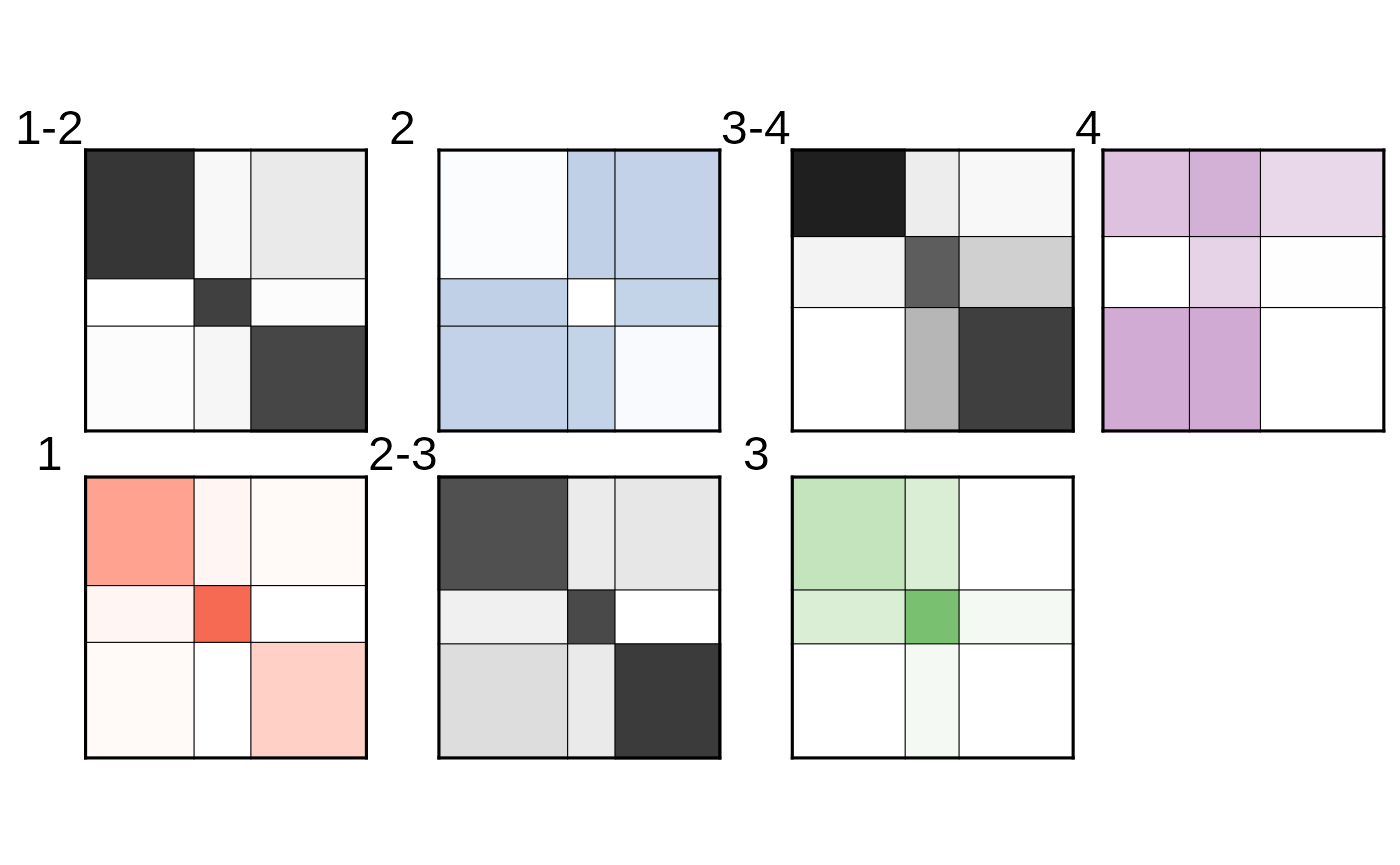
Or compared for each level, the inferred clustering with the simulated one with ARI (1 for perfect recovery, 0 for clustering by chance):
paste(
  "ARI for level", seq(L), ":",
  round(sapply(seq(L),
       function(l) ARI(x = gmlv$memberships[[l]],
                       y = fit_from_scratch$Z[[l]])), 2)
)
#> [1] "ARI for level 1 : 1"    "ARI for level 2 : 1"    "ARI for level 3 : 0.96"
#> [4] "ARI for level 4 : 1"
Or compare the inferred clustering from our two methods of inference with ARI: