Tutorial on plant pollinator data • colSBM

library(colSBM)
library(patchwork)
library(parallel)
data("dorebipartite")

Estimation with colSBM

We load a list of 15 plant-pollinator networks. They are binary undirected networks with different number of plant and pollinator species.

Networks benefiting from joint modelisation

First, we are going to model jointly the medan2002ld, medan2002rb networks, using the iid-colBiSBM model.

set.seed(1234, "L'Ecuyer-CMRG")
res_pp_iid <- estimate_colBiSBM(
  netlist = dorebipartite[7L:8L], # A list of networks
  colsbm_model = "iid", # The name of the model
  net_id = names(dorebipartite)[7L:8L], # Name of the networks
  nb_run = 2L, # Number of runs of the algorithm
  global_opts = list(
    verbosity = 1L,
    plot_detail = 0L,
    nb_cores = 2L,
    backend = "parallel"
  )
)
#> 
#> Merging the 2 models
#> After merging the 2 model runs, the criteria are the following:
#> 
#> vbound : 
#>       [,1] [,2] [,3] [,4] [,5]
#> [1,] -Inf -625 -620 -620 -Inf
#> [2,] -720 -614 -605 -Inf -Inf
#> [3,] -720 -606 -596 -Inf -Inf
#> [4,] -Inf -Inf -Inf -Inf -Inf
#> [5,] -Inf -Inf -Inf -Inf -Inf
#> [6,] -Inf -Inf -Inf -Inf -Inf 
#> 
#> ICL    : 
#>       [,1] [,2] [,3] [,4] [,5]
#> [1,] -729 -635 -642 -650 -Inf
#> [2,] -733 -653 -665 -Inf -Inf
#> [3,] -739 -671 -667 -Inf -Inf
#> [4,] -Inf -Inf -Inf -Inf -Inf
#> [5,] -Inf -Inf -Inf -Inf -Inf
#> [6,] -Inf -Inf -Inf -Inf -Inf 
#> 
#> BICL   : 
#>       [,1] [,2] [,3] [,4] [,5]
#> [1,] -729 -635 -636 -641 -Inf
#> [2,] -730 -634 -635 -Inf -Inf
#> [3,] -736 -636 -640 -Inf -Inf
#> [4,] -Inf -Inf -Inf -Inf -Inf
#> [5,] -Inf -Inf -Inf -Inf -Inf
#> [6,] -Inf -Inf -Inf -Inf -Inf 
#> 
#> Best fit at Q=( 2, 2 )
#> 
#> ==== Best fits criterion for the 2 networks. Computed in 0.397 secs ====
#> Sep BiSBM total BICL:  -640.6602
#> colBiSBM BICL: -633.8697
#> Joint modelisation preferred. With Q = ( 2, 2 ).
#> 
#> ==== Full computation performed in 15 secs ====

The output indicates that the collection benefits from a joint modelisation

Joint modelisation preferred

This is based on the BICL criterion.

We can look at how the variational bound and the model selection criteria evolve with the number of clusters. Here, the BICL criterion selects Q = 2, 2 blocks.

plot(res_pp_iid)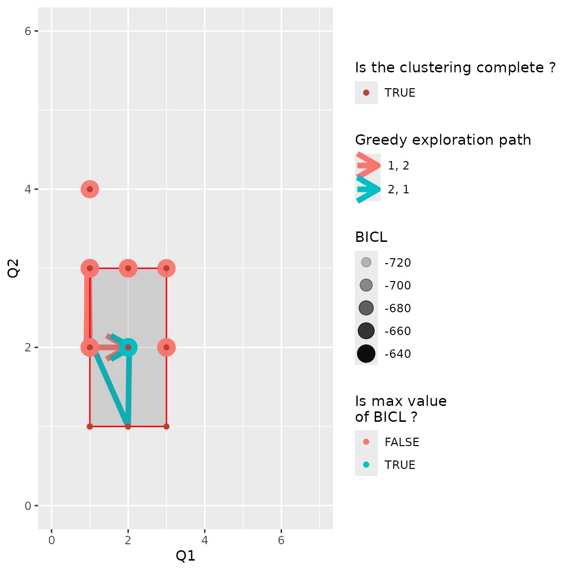

State-space exploration

best_fit <- res_pp_iid$best_fit

Results and analysis

Here are some useful fields to analyze the results.

best_fit
#> Fitted Collection of Bipartite SBM -- bernoulli variant for 2 networks 
#> =====================================================================
#> net_id = ( medan2002ld medan2002rb )
#> Dimensions = ( c(45, 21), c(72, 23) ) - ( 2, 2 ) blocks.
#> BICL =  -633.8697 
#> #Empty row blocks on all networks:  0  -- #Empty columns blocks on all networks:  0  
#> * Useful fields 
#>   $distribution, $nb_nodes, $nb_blocks, $support, $prob_memberships 
#>   $memberships, $parameters, $BICL, $vbound, $pred_dyads 
#> =====================================================================

We can retrieve:

the estimation of the model parameters

best_fit$parameters
#> $alpha
#>           [,1]       [,2]
#> [1,] 0.2132297 0.17088360
#> [2,] 0.4285972 0.03350959
#> 
#> $pi
#> $pi[[1]]
#> [1] 0.07572543 0.92427457
#> 
#> $pi[[2]]
#> [1] 0.07572543 0.92427457
#> 
#> 
#> $rho
#> $rho[[1]]
#> [1] 0.08387756 0.91612244
#> 
#> $rho[[2]]
#> [1] 0.08387756 0.91612244

The block memberships:

best_fit$memberships[[2]]$row[1:10]
#>        Birds Trochilidae Sappho sparganura 
#>                                          2 
#>     Coleoptera Buprestidae Buprestidae sp. 
#>                                          2 
#>     Coleoptera Cantharidae Cantharidae sp. 
#>                                          2 
#>  Coleoptera Coccinellidae Coccinelidae sp1 
#>                                          2 
#>  Coleoptera Coccinellidae Coccinelidae sp2 
#>                                          2 
#>  Coleoptera Coccinellidae Coccinelidae sp3 
#>                                          2 
#> Coleoptera Curculionidae Curculionidae sp. 
#>                                          2 
#>           Coleoptera Meloidae Epicauta sp. 
#>                                          2 
#>     Coleoptera Mordellidae Mordellidae sp. 
#>                                          2 
#>      Diptera Anthomyiidae Anthomyiidae sp2 
#>                                          2

And their probabilities:

best_fit$prob_memberships[[2]][[1]][1:10, 1]
#>        Birds Trochilidae Sappho sparganura 
#>                               0.2000449903 
#>     Coleoptera Buprestidae Buprestidae sp. 
#>                               0.0148961299 
#>     Coleoptera Cantharidae Cantharidae sp. 
#>                               0.0026079747 
#>  Coleoptera Coccinellidae Coccinelidae sp1 
#>                               0.0009135321 
#>  Coleoptera Coccinellidae Coccinelidae sp2 
#>                               0.0026079747 
#>  Coleoptera Coccinellidae Coccinelidae sp3 
#>                               0.0026079747 
#> Coleoptera Curculionidae Curculionidae sp. 
#>                               0.0026079747 
#>           Coleoptera Meloidae Epicauta sp. 
#>                               0.0414498548 
#>     Coleoptera Mordellidae Mordellidae sp. 
#>                               0.0009135321 
#>      Diptera Anthomyiidae Anthomyiidae sp2 
#>                               0.0026079747

The prediction for each dyads in the networks

best_fit$pred_dyads[[2]][1:10, 1]
#>        Birds Trochilidae Sappho sparganura 
#>                                 0.06144805 
#>     Coleoptera Buprestidae Buprestidae sp. 
#>                                 0.03610547 
#>     Coleoptera Cantharidae Cantharidae sp. 
#>                                 0.03442351 
#>  Coleoptera Coccinellidae Coccinelidae sp1 
#>                                 0.03419158 
#>  Coleoptera Coccinellidae Coccinelidae sp2 
#>                                 0.03442351 
#>  Coleoptera Coccinellidae Coccinelidae sp3 
#>                                 0.03442351 
#> Coleoptera Curculionidae Curculionidae sp. 
#>                                 0.03442351 
#>           Coleoptera Meloidae Epicauta sp. 
#>                                 0.03974006 
#>     Coleoptera Mordellidae Mordellidae sp. 
#>                                 0.03419158 
#>      Diptera Anthomyiidae Anthomyiidae sp2 
#>                                 0.03442351

We can also plot the networks individually:

plot(res_pp_iid$best_fit, type = "block", net_id = 1) +
  plot(res_pp_iid$best_fit, type = "block", net_id = 2)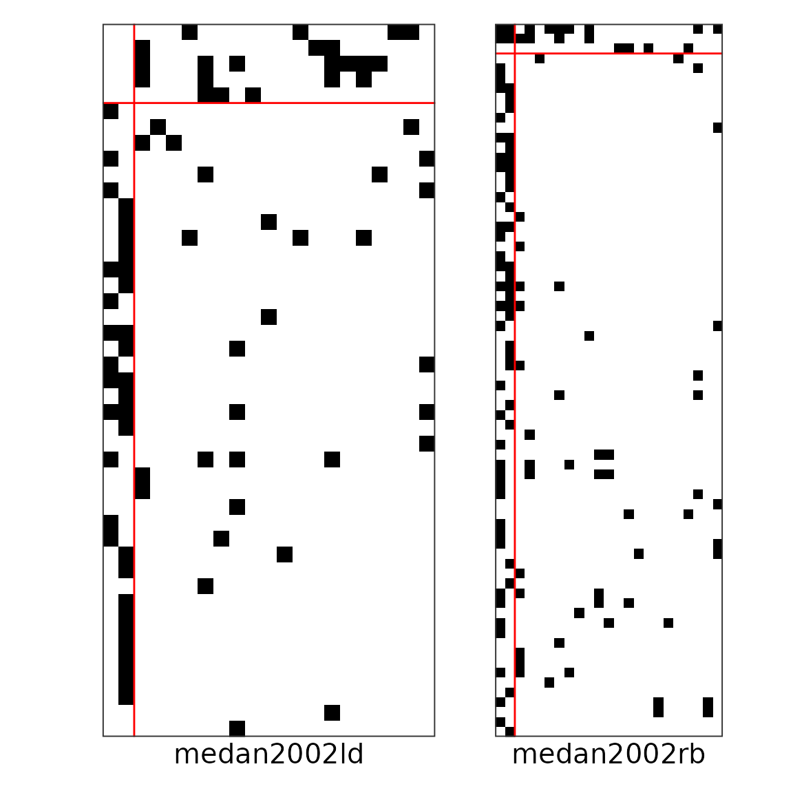

Networks after fitting the model and reordering the nodes and blocks

Or make different plots to exhibit the mesoscale structure:

plot(res_pp_iid$best_fit, type = "graphon")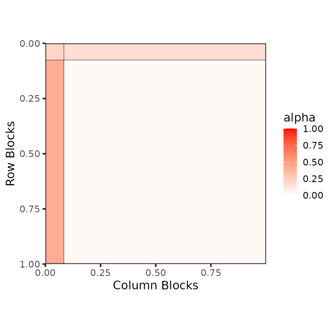

Graphon type plot

plot(res_pp_iid$best_fit, type = "meso", mixture = TRUE)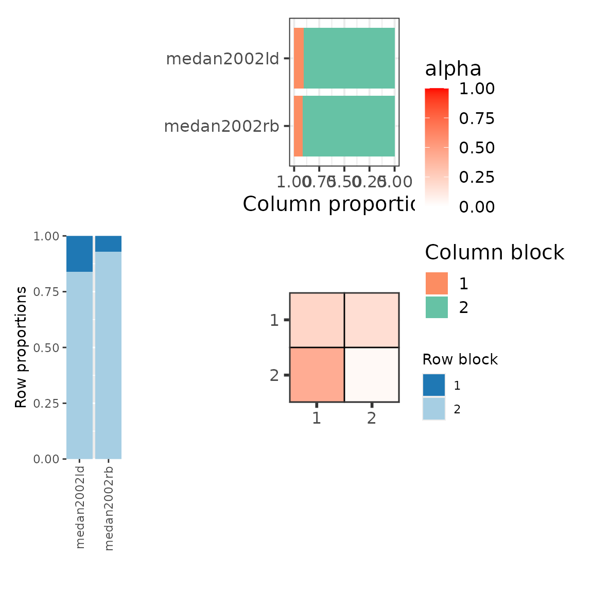

Mesoscale type plot

Networks not benefiting from joint modelisation

Next, we model jointly the medan2002ld, medan2002rb, olensen2002aig, olensen2002flo networks, using the iid-colBiSBM model.

res_pp_iid_sep <- estimate_colBiSBM(
  netlist = dorebipartite[7L:10L], # A list of networks
  colsbm_model = "iid", # The name of the model
  net_id = names(dorebipartite)[7L:10L], # Name of the networks
  nb_run = 1L, # Number of runs of the algorithm
  global_opts = list(
    verbosity = 1L,
    plot_detail = 0L,
    nb_cores = 2L,
    backend = "no_mc"
  )
)
#> 
#> 
#> 
#> 
#> 
#> ==== Best fits criterion for the 4 networks. Computed in 1.09 secs ====
#> Sep BiSBM total BICL:  -813.0666
#> colBiSBM BICL: -817.1685
#> Separated modelisation preferred.
#> 
#> ==== Full computation performed in 7.76 secs ====

The output indicates that the collection does not benefit from a joint modelisation.

Separated modelisation preferred

The structures might be too different to be gathered in one collection.

Clustering of networks

In the case of different structures clustering can be used to find a partitionning among all the networks.

We will simulate networks and add them to the 4 networks we used previously.

alpha <- matrix(c(
  0.9, 0.55,
  0.6, 0.1
), 2, 2, byrow = TRUE)
pi <- c(0.73, 0.27)
rho <- c(0.75, 0.25)
sim_net <-
  generate_bipartite_collection(
    nr = 40L,
    nc = 30L,
    pi = pi,
    rho = rho,
    alpha = alpha,
    M = 2L,
    model = "iid"
  )

set.seed(1234L)
net_clust <- clusterize_bipartite_networks(
  netlist = c(dorebipartite[7L:10L], sim_net), # A list of networks
  colsbm_model = "iid", # The name of the model
  net_id = c(
    names(dorebipartite)[7L:10L],
    paste0("sim", seq_along(sim_net))
  ), # Name of the networks
  nb_run = 1L, # Number of runs of the algorithm
  global_opts = list(
    verbosity = 0L,
    plot_details = 0L,
    nb_cores = 2L,
    backend = "no_mc",
    Q1_max = 9L,
    Q2_max = 9L
  ), # Max number of clusters
  fit_opts = list(max_vem_steps = 1000L)
)

best_partition <- extract_best_partition(net_clust)

We obtain a list of 3 tested collections. The lists are nested and reflect the sequential steps of clustering. The extraction of the best partition below reveals that our 2 simulated networks are considered as being part of the same collection and that the among the 4 plant-pollinator networks there exists a difference leading to 2 collections that contains networks from the same authors.

The plot of the mesoscale structure of the whole collection (ie before partitionning) is the following:

plot(net_clust[[1]])

Whole collection graphon type plot

but then we can compare the mesoscale structures of the 3 groups:

wrap_plots(
  lapply(best_partition, function(collection) {
    plot(collection, type = "graphon") +
      ggplot2::ggtitle(label = "", subtitle = toString(collection$net_id))
  }),
  ncol = 2L
)

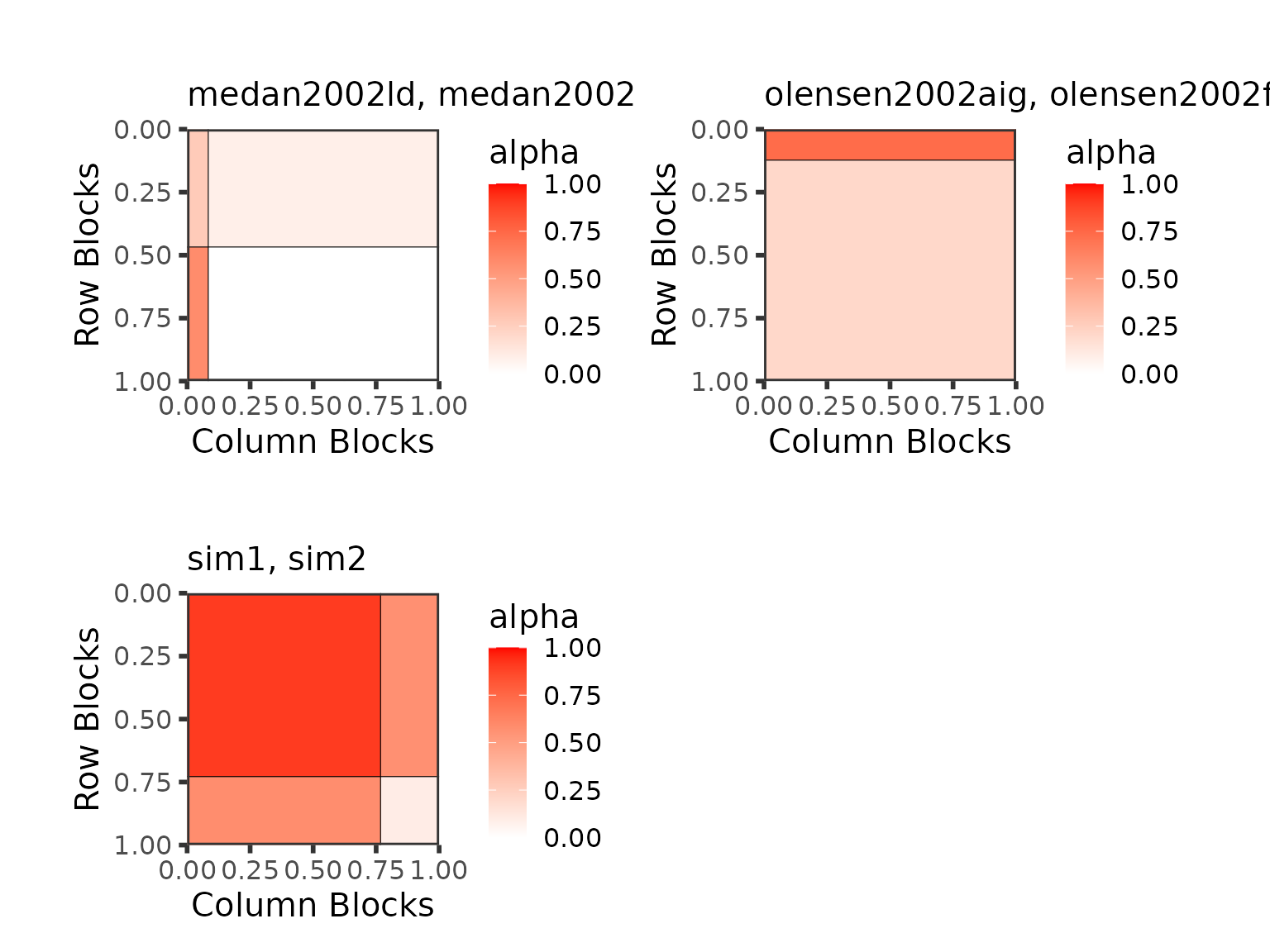
Best partition graphon type plots