Tutorial on food webs
tutorial.RmdEstimation with colSBM
We load a list of 8 foodwebs. They are binary directed networks with different number of species. First, we are going to model jointly the first networks, using the iid-colSBM model.
# global_opts = list(nb_cores = 1L,
#                    nb_models = 5L,
#                    nb_init = 10L,
#                    depth = 2L,
#                    verbosity = 1,
#                    spectral_init = FALSE,
#                    Q_max = 8L,
#                    plot_details = 1)

set.seed(1234)
res_fw_iid <- estimate_colSBM(
  netlist = foodwebs[1:3], # A list of networks
  colsbm_model = "iid", # The name of the model
  directed = TRUE, # Foodwebs are directed networks
  net_id = names(foodwebs)[1:3], # Name of the networks
  nb_run = 1L, # Number of runs of the algorithm
  global_opts = list(
    verbosity = 0,
    plot_details = 0,
    Q_max = 8
  ) # Max number of clusters
)
We can look at how the variational bound and the model selection criteria evolve with the number of clusters. Here, the BICL criterion selects Q = 6 blocks.
plot(res_fw_iid)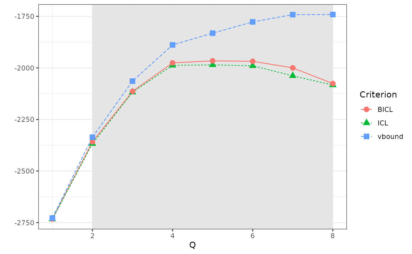
best_fit <- res_fw_iid$best_fitResults and analysis
Here are some useful fields to analyze the results.
best_fit
#> Fitted Collection of Simple SBM -- bernoulli variant for 3 networks
#> =====================================================================
#> Dimension = ( 105 58 71 ) - ( 6 ) blocks.
#> BICL =  -1967.254  -- #Empty blocks :  0
#> =====================================================================
#> * Useful fields
#>   $distribution, $nb_nodes, $nb_clusters, $support, $Z
#>   $memberships, $parameters, $BICL, $vbound, $pred_dyads
We can get:
- the estimation of the model parameters
best_fit$parameters
#> $alpha
#>              [,1]         [,2]         [,3]         [,4]         [,5]
#> [1,] 1.337284e-03 1.855419e-10 0.0379944789 1.036529e-11 4.232057e-06
#> [2,] 7.125890e-01 2.916621e-08 0.5523050570 9.448324e-10 8.086073e-01
#> [3,] 1.422084e-05 9.845693e-11 0.0342935378 6.575492e-12 2.697802e-09
#> [4,] 2.019119e-02 1.434655e-09 0.0005668503 7.879153e-11 1.866794e-01
#> [5,] 5.387169e-06 4.879625e-10 0.1275977515 7.992381e-04 9.099859e-10
#> [6,] 7.400179e-02 2.978761e-09 0.4974226156 5.319729e-10 1.534667e-04
#>              [,6]
#> [1,] 2.052649e-02
#> [2,] 7.996047e-01
#> [3,] 3.464961e-07
#> [4,] 7.360008e-02
#> [5,] 1.820506e-02
#> [6,] 1.987907e-01
#>
#> $pi
#> $pi[[1]]
#> [1] 0.24801191 0.02564113 0.07861710 0.45691659 0.13378060 0.05703266
#>
#> $pi[[2]]
#> [1] 0.24801191 0.02564113 0.07861710 0.45691659 0.13378060 0.05703266
#>
#> $pi[[3]]
#> [1] 0.24801191 0.02564113 0.07861710 0.45691659 0.13378060 0.05703266
#>
#>
#> $delta
#> [1] 1 1 1- The block memberships:
best_fit$Z
#> [[1]]
#> Unidentified sp1 FW_009 Terrestrial plant material
#> 2 2
#> Terrestrial invertebrates Achnanthes lanceolata
#> 6 4
#> Batrachospermum Calothrix sp1 FW_009
#> 4 4
#> Cocconeis placentula Cosmarium sp1 FW_009
#> 4 4
#> Cyclotella sp1 FW_009 Cymbella aspera
#> 4 4
#> Cymbella cuspidata Cymbella kappi
#> 4 4
#> Cymbella tumida Diatoma heimale
#> 4 4
#> Epithemia sorex Epithemia turgida
#> 4 4
#> Eunotia serpentina Unidentified sp2 FW_009
#> 4 4
#> Euntoia pectinalis Fragilaria sp1 FW_009
#> 4 4
#> Fragilaria vaucheriae Frustulia rhomboides
#> 4 4
#> Gomphoneis herculeana Gomphonema accuminatum
#> 4 4
#> Gomphonema angustatum Gomphonema truncatum
#> 4 4
#> Unidentified sp3 FW_009 Melosira varians
#> 4 4
#> Navicula avenacea Navicula dicephala
#> 4 4
#> Nitzschia dubia Oedogonium sp1 FW_009
#> 4 4
#> Phormidium sp1 FW_009 Pinnularia mesolepta
#> 4 4
#> Pinnularia viridis Pleaurotaenium sp1 FW_009
#> 4 4
#> Rhoicospenia curvata Rhopalodia sp1 FW_009
#> 4 4
#> Schizothrix sp1 FW_009 Staurastrum sp1 FW_009
#> 4 4
#> Surirella elegans Surirella tenera
#> 4 4
#> Synedra ulna Tabellaria fenestrata
#> 4 4
#> Tabellaria flocculosa Ulothrix sp1 FW_009
#> 4 4
#> Unidentified sp4 FW_009 Unidentified sp5 FW_009
#> 4 4
#> Acroneuria sp1 FW_009 Aelosoma sp1 FW_009
#> 3 6
#> Alloperla sp1 FW_009 Anepeorus sp1 FW_009
#> 4 3
#> Antocha saxicola Baetis
#> 1 5
#> Boyeria vinosa Bryophaenocladius sp1 FW_009
#> 1 1
#> Chauliodes sp1 FW_009 Chimarra atterima
#> 3 6
#> Unidentified sp6 FW_009 Conchapelopia sp1 FW_009
#> 5 6
#> Cryptolabis sp1 FW_009 Cyrnellus sp1 FW_009
#> 1 1
#> Dicrotendipes sp1 FW_009 Diplectrona modesta
#> 5 5
#> Ectopria nervosa Endochironomous sp1 FW_009
#> 5 6
#> Ephemerella sp1 FW_009 Eukieferiella pseudomontana
#> 1 1
#> Eukiefferiella 'dark' type Glossosoma sp1 FW_009
#> 5 1
#> Gyraulus sp1 FW_009 Haploperla brevis
#> 5 1
#> Hexatoma sp1 FW_009 Hydrophilidae
#> 3 1
#> Hydropsyche sp1 FW_009arana Larsia sp1 FW_009
#> 6 1
#> Leucrocuta sp1 FW_009 Leuctra sp1 FW_009
#> 5 5
#> Unidentified sp7 FW_009 Metriocnemus sp1 FW_009
#> 6 5
#> Micrasema sp1 FW_009 Ochthebius sp1 FW_009
#> 1 1
#> Ophiogomphus sp1 FW_009 Paraleptophlebia sp1 FW_009
#> 3 1
#> Paranyctiophylax sp1 FW_009 Polycentropus sp1 FW_009
#> 1 1
#> Probezzia sp1 FW_009 Promoresia sp1 FW_009
#> 1 5
#> Psephenus sp1 FW_009 Pseudolimnolphila sp1 FW_009
#> 5 1
#> Rhyacophila sp1 FW_009 Simulium sp1 FW_009
#> 1 5
#> Sphaerium occidentale Stempelinella sp1 FW_009
#> 1 5
#> Stenelmis crenata Stenelmis sp1 FW_009
#> 5 5
#> Suwalia sp1 FW_009 Tallaperla sp1 FW_009
#> 1 6
#> Tanytarsus Genus A Tricorythodes sp1 FW_009
#> 1 1
#> Notropis heterolepsis Brook trout
#> 3 3
#> Orcnocetes virilis Rhinichthys cataractae
#> 1 3
#> Cambarus bartonii
#> 1
#>
#> [[2]]
#> Unidentified sp1 FW_012_01 Terrestrial invertebrates
#> 2 4
#> Plant material Achnanthes lanceolata
#> 2 4
#> Achnanthes minutissima Audouinella sp1 FW_012_01
#> 4 4
#> Batrachospermum Blue-green algae
#> 4 4
#> Calothrix Cymbella cistula
#> 4 4
#> Cymbella mulleri Diatoma heimale
#> 4 4
#> Epithemia sorex Epithemia turgida
#> 4 4
#> Eunotia pectinalis Eunotia sp1 FW_012_01
#> 4 4
#> Frustulia rhomboides Gomphoneis herculeana
#> 4 4
#> Gomphonema intricatum Gomphonema sp1 FW_012_01
#> 4 4
#> Meridion circulare Navicula avenacea
#> 4 4
#> Pleurotaenium Rhoicosphenia curvata
#> 4 4
#> Stigeoclonium Synedra ulna
#> 4 4
#> Ulothrix Unidentified sp2 FW_012_01
#> 4 4
#> Aelosoma Brachycentrus sp1 FW_012_01
#> 6 5
#> Cambarus bartoni Chauliodes sp1 FW_012_01
#> 3 1
#> Cordulegaster maculata Dicranota sp1 FW_012_01
#> 1 1
#> Ectopria thoracica Epeorus dispar
#> 5 5
#> Glossosoma sp1 FW_012_01 Homoplectra sp1 FW_012_01
#> 1 1
#> Hudsonimya sp1 FW_012_01 Hydropsyche sp1 FW_012_01
#> 1 6
#> Leucrocuta sp1 FW_012_01 Leuctra sp1 FW_012_01
#> 5 1
#> Lumbriculiid oligochaete Parametriocnemus sp1 FW_012_01
#> 6 5
#> Neureclipsis sp1 FW_012_01 Ophiogomphus sp1 FW_012_01
#> 1 1
#> Palpomyia sp1 FW_012_01 Palpomyia sp2 FW_012_01
#> 1 1
#> Promoresia sp1 FW_012_01 Psephenus sp1 FW_012_01
#> 5 5
#> Soliperla sp1 FW_012_01 Stenelmis adult
#> 3 1
#> Stenelmis sp1 FW_012_01 Suwalia sp1 FW_012_01
#> 1 3
#> Tallaperla maria Thaumalea sp1 FW_012_01
#> 1 5
#> Tipula abdominalis Salamander
#> 1 3
#>
#> [[3]]
#> Unidentified sp1 FW_012_02 Terrestrial plants
#> 2 2
#> Terrestrial bugs Achnanthes inflata var. elata
#> 1 4
#> Achnanthes lanceolata Achnanthes linearis
#> 4 4
#> Achnanthes minutissima Auodinella hermanii
#> 4 4
#> Blue Green algae Calothrix
#> 4 4
#> Cocconeis placentula Cymbella kappi
#> 4 4
#> Cymbella mulleri Diatoma heimale
#> 4 4
#> Epithemia turgida Eunotia meisteri
#> 4 4
#> Eunotia pectinalis Fragilaria vaucheriae
#> 4 4
#> Frustulia rhomboides Gomphoneis herculeana
#> 4 4
#> Gomphonema accuminatum Gomphonema angustatum
#> 4 4
#> Gomphonema intricatum Gomphonema tennuellum
#> 4 4
#> Marssoniella Navicula avenacea
#> 4 4
#> Navicula cryptocephala Navicula mutica
#> 4 4
#> Navicula sp1 FW_012_02 Pinnularia viridis
#> 4 4
#> Rhoicosphenia curvata Rhopalodia
#> 4 4
#> Surirella brebbisonii Surirella elegans
#> 4 4
#> Synechoccus Synedra ulna
#> 4 4
#> Ulothrix Unidentified sp2 FW_012_02
#> 4 4
#> Aeolosoma sp1 FW_012_02 Ajax longipes
#> 6 3
#> Amphinemura wui Anchytarsus bicolor
#> 1 1
#> Baetis Hudsonimya
#> 5 1
#> Cricotopus Dicranota
#> 5 1
#> Eukieffidrella pseudomontana Diplectrona modesta
#> 1 1
#> Dixella Dolophilodes
#> 1 3
#> Ectopria thoracica Epeorus dispar
#> 5 5
#> Fatigia pele Hexatoma sp1 FW_012_02
#> 1 3
#> Leuctra Oligo Lumbr. Blue
#> 5 5
#> Oligo. Lumbr. Pink Ophiogomphus
#> 1 1
#> Paraleptophelebia Pericoma
#> 1 1
#> Pilaria Pentaneuri sp1 FW_012_02
#> 1 1
#> Polycentropus maculatus Stenelmis
#> 1 5
#> Tallaperla maria Tanyderid
#> 1 1
#> Conchapelopia Tipula
#> 1 1
#> Wormaldia moesta Crayfish
#> 1 3
#> Salamander
#> 3- The prediction for each dyads in the networks, here for network
number 3. If your goal is dyad prediction, then you should use
colsbm_model = "delta", instead ofcolsbm_model = "iid".
best_fit$pred_dyads[[3]][1:10, 1:5]
#>                               Unidentified sp1 FW_012_02 Terrestrial plants
#> Unidentified sp1 FW_012_02                  0.000000e+00       3.203932e-08
#> Terrestrial plants                          3.203932e-08       0.000000e+00
#> Terrestrial bugs                            5.150140e-10       5.150140e-10
#> Achnanthes inflata var. elata               1.715692e-09       1.715692e-09
#> Achnanthes lanceolata                       1.715692e-09       1.715692e-09
#> Achnanthes linearis                         1.715692e-09       1.715692e-09
#> Achnanthes minutissima                      1.715692e-09       1.715692e-09
#> Auodinella hermanii                         1.704351e-09       1.704351e-09
#> Blue Green algae                            1.715692e-09       1.715692e-09
#> Calothrix                                   1.715693e-09       1.715693e-09
#>                               Terrestrial bugs Achnanthes inflata var. elata
#> Unidentified sp1 FW_012_02          0.62896381                  5.117223e-08
#> Terrestrial plants                  0.62896381                  5.117223e-08
#> Terrestrial bugs                    0.00000000                  2.653609e-08
#> Achnanthes inflata var. elata       0.01914963                  0.000000e+00
#> Achnanthes lanceolata               0.01914963                  2.608635e-09
#> Achnanthes linearis                 0.01914963                  2.608635e-09
#> Achnanthes minutissima              0.01914963                  2.608635e-09
#> Auodinella hermanii                 0.01901584                  2.601152e-09
#> Blue Green algae                    0.01914963                  2.608635e-09
#> Calothrix                           0.01914963                  2.608635e-09
#>                               Achnanthes lanceolata
#> Unidentified sp1 FW_012_02             3.818738e-09
#> Terrestrial plants                     3.818738e-09
#> Terrestrial bugs                       2.571672e-08
#> Achnanthes inflata var. elata          3.606283e-10
#> Achnanthes lanceolata                  0.000000e+00
#> Achnanthes linearis                    3.606283e-10
#> Achnanthes minutissima                 3.606283e-10
#> Auodinella hermanii                    3.671654e-10
#> Blue Green algae                       3.606283e-10
#> Calothrix                              3.606284e-10
We can also plot the networks individually, with the groups reordered by trophic levels:
p <- gtools::permutations(best_fit$Q, best_fit$Q)
ind <- which.min(
  sapply(
    seq(nrow(p)),
    function(x) {
      sum((tcrossprod(best_fit$pi[[1]]) * best_fit$alpha)[p[x, ], p[x, ]][
        upper.tri(best_fit$alpha)
      ])
    }
  )
)
ord <- p[ind, ]
plot(res_fw_iid$best_fit, type = "block", net_id = 1, ord = ord) +
  plot(res_fw_iid$best_fit, type = "block", net_id = 2, ord = ord) +
  plot(res_fw_iid$best_fit, type = "block", net_id = 3, ord = ord)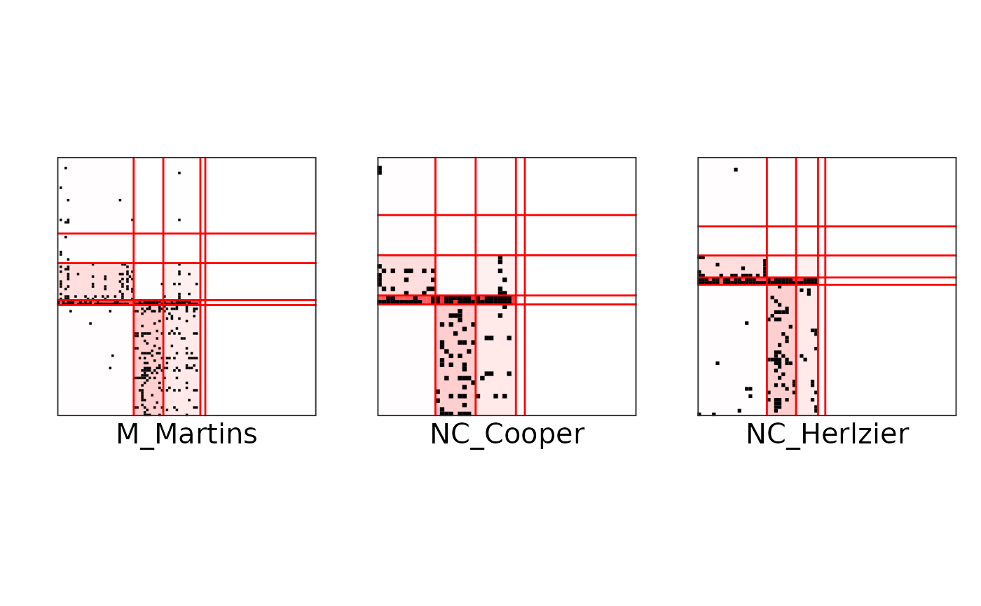
Or make different plots to exhibit the mesoscale structure:
plot(res_fw_iid$best_fit, type = "graphon", ord = ord)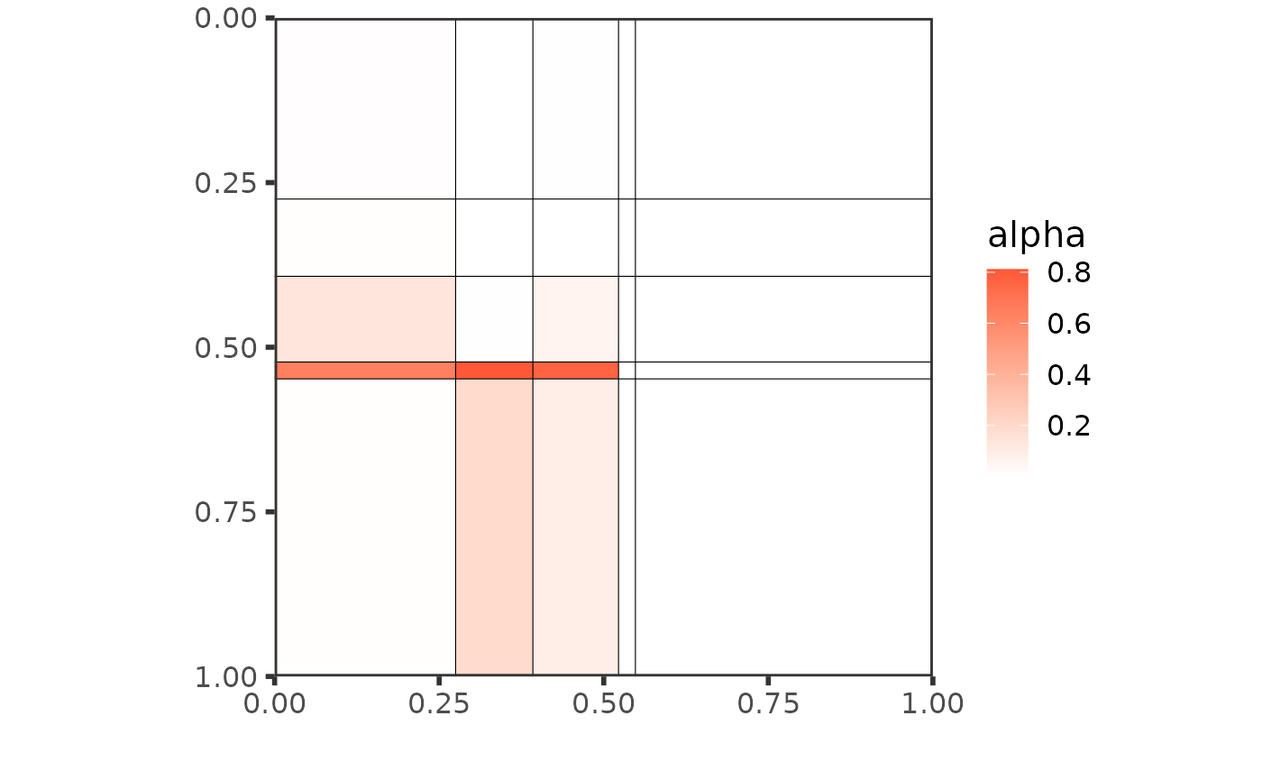
plot(res_fw_iid$best_fit, type = "meso", mixture = TRUE, ord = ord)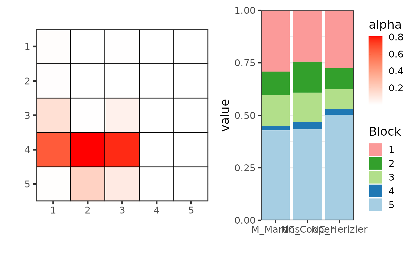
Clustering of networks
Let simulate some directed networks with a lower triangular structure that looks alike foodwebs.
set.seed(1234)
alpha <- matrix(c(
  .05, .01, .01, .01,
  .3, .05, .01, .01,
  .5, .4, .05, .01,
  .1, .8, .1, .05
), 4, 4, byrow = TRUE)
pi <- c(.1, .2, .6, .1)
sim_net <-
  replicate(3,
    {
      X <-
        sbm::sampleSimpleSBM(100,
          blockProp = pi, connectParam = list(mean = alpha),
          directed = TRUE
        )
      X$rNetwork
      X$networkData
    },
    simplify = FALSE
  )
set.seed(1234)

net_clust <- clusterize_unipartite_networks(
  netlist = c(foodwebs[1:3], sim_net), # A list of networks
  colsbm_model = "iid", # The name of the model
  directed = TRUE, # Foodwebs are directed networks
  net_id = c(names(foodwebs)[1:3], "sim1", "sim2", "sim3"), # Name of the networks
  nb_run = 3L, # Nmber of runs of the algorithm
  global_opts = # List of options
    list(
      verbosity = 0, # Verbosity level of the algorithm
      plot_details = 0, # Monitoring plot of the algorithm
      Q_max = 9, # Max number of clusters
      backend = "parallel" # Backend for parallel computing
    ),
  verbose = FALSE
)
We can extract the best partition:
best_partition <- net_clust$partitionThe plot of the mesoscale structure of the whole collection is the following:
plot(best_partition[[1]])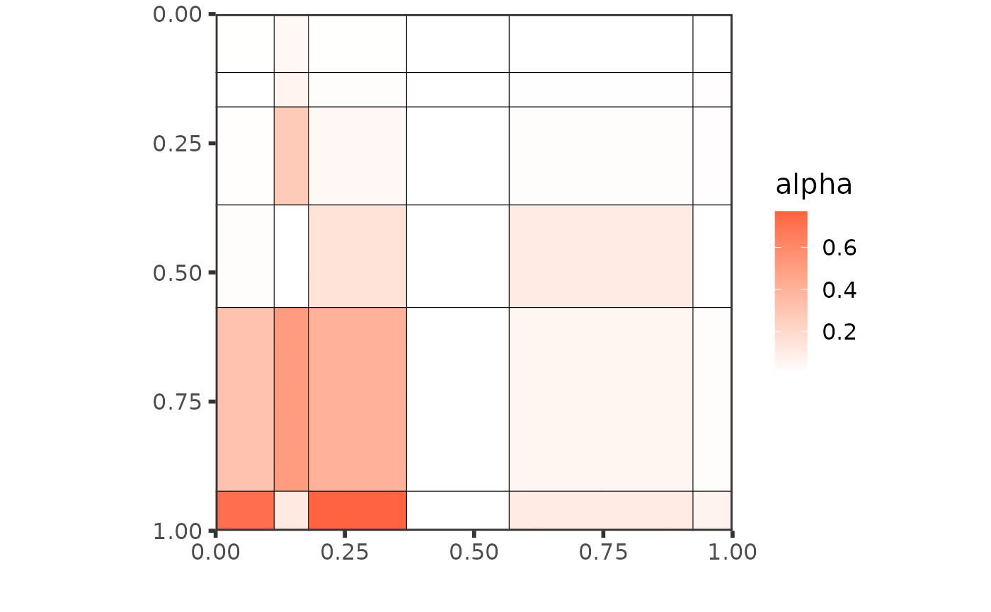
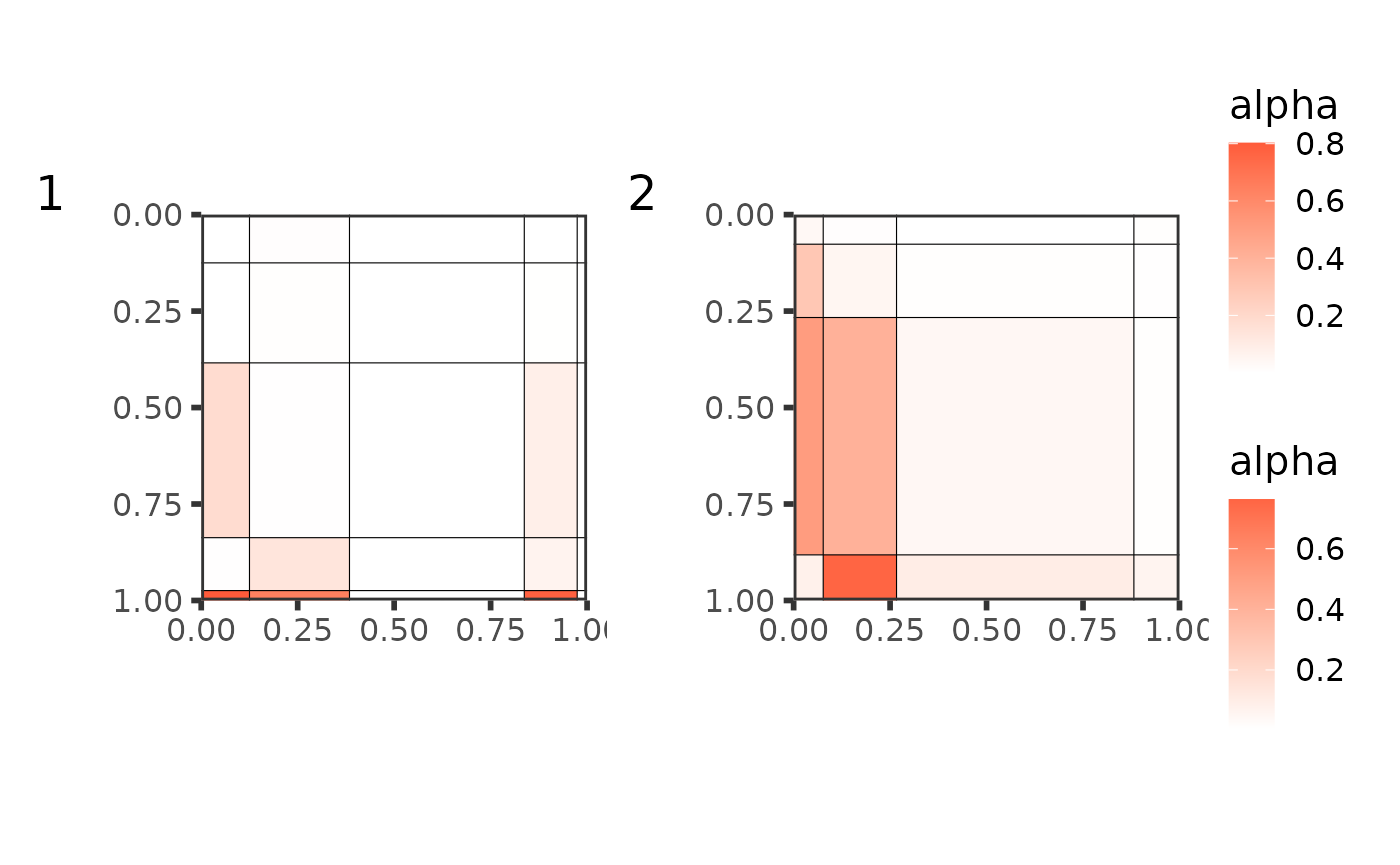
but then we can compare the mesoscale structures of the 2 groups:
plot(best_partition[[1]],
  type = "graphon",
  ord = order(best_partition[[1]]$alpha %*% best_partition[[1]]$pi[[1]])
) +
  plot(best_partition[[2]],
    type = "graphon",
    ord = order(best_partition[[2]]$alpha %*% best_partition[[2]]$pi[[1]])
  ) +
  plot_layout(guides = "collect") + plot_annotation(tag_levels = "1")